

EC‐MS Application Note #1
CO‐stripping Technique
EC‐MS Application Note #1
- Last updated

Why Do a CO‐strip?
*CO + H2O → CO2 + 2 H+ + 2 e–
Experimental Procedure for CO-strip
Safety & Experimental Considerations
Reference Measurement
Start by setting up experimental parameters in Zilien and EC-lab. The experimental procedure in EC-lab should contain a CVA technique followed by a loop. Choose suitable values of parameters such as current range, bandwidth, scan rate etc. depending on the experiment and system studied. For further detail on EC parameters consult the EC-lab manual and application notes, as well as EC-MS Technical Note #3. Pump down the chip and start the Zilien experiment. Set a flow of 1 mL/min inert make-up gas (e.g. He) on line #1 via MFC1. Prior to starting EC experiments, perform a breath test and a drop test to verify that the EC-MS is fully operational. Mount cell with sample, inject electrolyte and connect glass pipes and electrode connections. For more details on preparation steps above, see the EC-MS manual. Make a reference measurement:
(i) Trigger the EC experiment from Zilien and wait to obtain a stable CV. Use the same set of parameters in EC-lab that will be used during the CO-strip for comparison (scan speed, potential limits etc.).
(ii) Obtain the reference measurement: First, end the CV with a potential hold at +0.05 V vs. RHE for 10 min.
(iii) Then start cycling the potential again (using the loop to restart the CVA technique). The first cycle can be used as a baseline for background subtraction during data treatment.
Gas Exchange to Induce CO-poisoning
Next, CO is introduced to the cell to induce CO-poisoning. Keep the same Zilien and EC-lab measurements running that were used for the baseline measurement. Before switching gases, ensure the inlet valve on the CO line is open (i.e. V9 when line #2 is used for CO) and the MFC2 mode is normal. Now perform the gas exchange:
(i) End the CV with a potential hold at +0.05 V vs. RHE.
(ii) Write 10 mL/min in the MFC2 setpoint field but do not press enter or click outside the field.
(iii) In quick succession click V8 and write and enter 0 mL/min in the MFC1 setpoint field. This connects line #2 to the chip while initializing a 10 mL/min flow of CO, while line #1 is closed and the He flow is stopped. Now CO enters the chip and saturates the electrolyte. The M28 signal seen in the MID will promptly increase while M4 decreases, as seen in the top panel of Fig. 1a. Simultaneously, a peak is observed in the current (red trace, bottom panel) due to CO displacing adsorbed hydrogen on the Pt electrode.
(iv) When the M28 signal stabilizes at a maximum, the make-up gas can be switched back to the inert gas: write but do not enter 10 mL/min in the MFC1 setpoint field. In quick succession click on V8 and write and enter 0 mL/min in the MFC2 setpoint field.
(v) Keep an eye on the pressure at P3 when running gas flows at 10 mL/min. If P3 is higher than expected, the gas ballast on the scroll pump should be used. After a few minutes the He flow can be turned down to 1 mL/min.
(vi) If the CO gas is no longer required in this measurement the MFC2 mode can be set to Flow Off and the inlet valve closed (e.g. V9 when line #2 is used for CO). If instead a different gas is desired on line #2, the entire line (all the way through MFC2) should be pumped via the gas manifold.
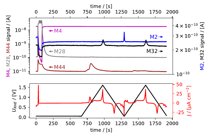
(a) EC‐MS plot during gas exchange and CO‐strip as a function of time
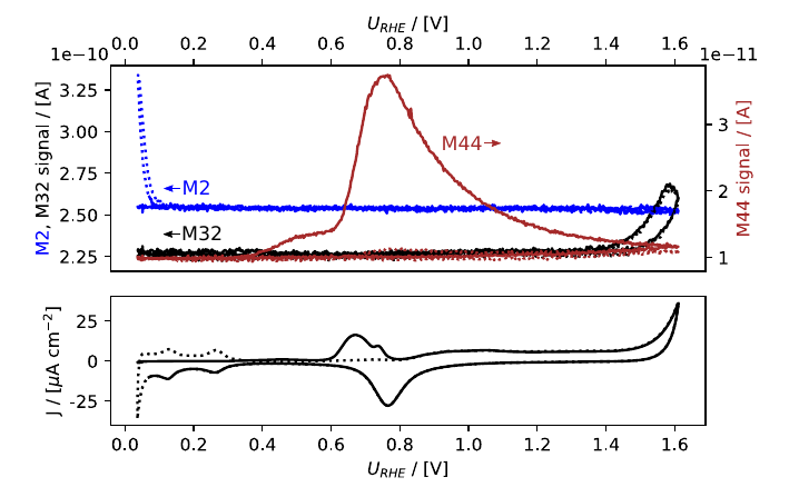
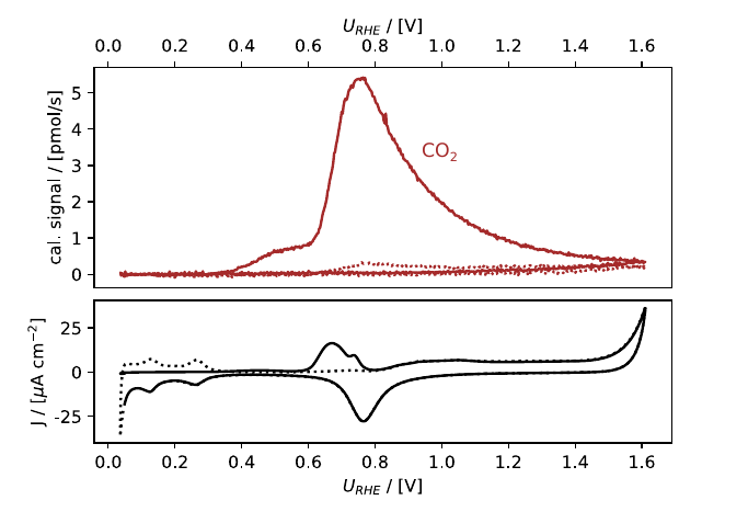
Figure 1: EC-MS plot during gas exchange and CO-strip. Mass spectrometer signals are shown in the top panels, electrochemical potential vs. RHE and current density in the bottom panels. (a) Initially, the potential is held at +50 mV vs. RHE while the make-up gas is changed from He to CO, as seen in the M4 and M28 signals. A sharp peak in the current density (red) is observed immediately, due to CO displacing adsorbed hydrogen on the Pt sample. The potential is held constant while switching the make-up gas back to He until all non-adsorbed CO is purged out. Upon sweeping the potential (5 mV/s scan rate) anodically, a peak in the electrochemical current and the M44 signal are observed, indicating the oxidation of adsorbed CO to CO2. (b) shows the CVs as a function of potential. The second cycle from (a) is shown as baseline (dotted).
CO Strip
Data Treatment
Surface Area Determination
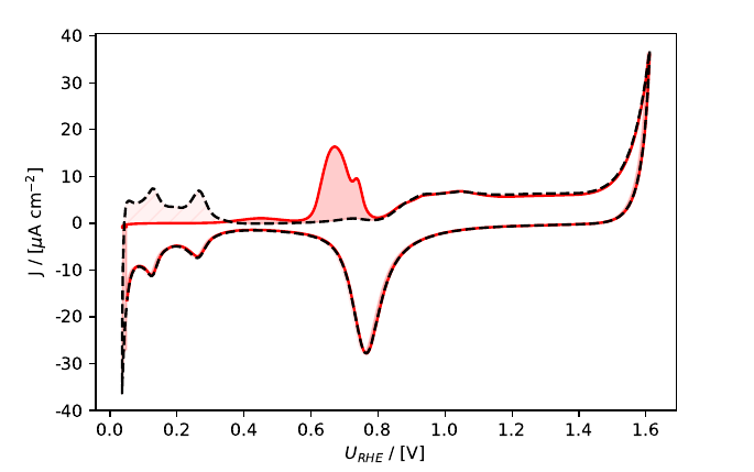
ECSA = (QCO-strip − Qref) [µC] / 340 [µC cm-2]
CO2 Calibration
As mentioned, the faradaic current observed during the CO-strip is related to the number of molecules of CO being oxidized according to Faraday’s law of electrolysis, where Q is the total charge, z the number of electrons in the reaction (z = 2 in the case of CO oxidation) and F the Faraday constant:
Due to the design of the EC-MS chip, all CO2 formed during the CO strip will be observed in the MS, which means that the faradaic current can be used to calibrate the MS signal of CO2 to convert from detector current IMS in [A] to molecular flux ṅCO2 in [mol/s]:
ṅCO2 [mol/s] = IMS [A] / FCO2,M44 [C/mol]
Where FCO2,M44 is the calibration factor for CO2 measured at m/z = 44 (M44), according to eq. 5:
FCO2,M44 [C/mol] = QM44 [A s] / ṅCO2,EC [mol]
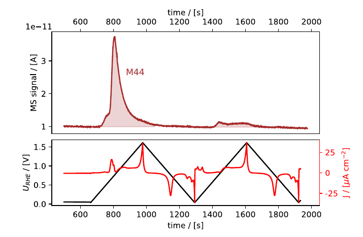
Figure 3: EC-MS plot highlighting the integrated CO2 signal from the CO-strip shown in Fig. 1a. Note that the baseline is not at 0 A, therefore a suitable baseline level should be chosen for the integration.
References
All data treatment and plotting in this application note was carried out using the open source Python package ixdat, available at https://github.com/ixdat/ixdat.