

EC‐MS Application Note #2
Quantification using ixdat
EC‐MS Application Note #2
- Last updated

Introduction
Quantified mass spectrometry data allows for the determination of faradaic efficiencies of reaction products, surface coverage and other important quantities which can help elucidating electrochemical processes. To obtain quantitative information, the current measured by the detector of the mass spectrometer (MS) needs to be related to the number of a certain type of molecules present at the vacuum inlet – i.e. the membrane chip in case of the EC-MS. Upon ionisation in the mass spectrometer, a significant amount of energy is introduced into the molecules, which leads to bonds breaking and molecular fragmentation. Each molecule presents with a typical cracking pattern at a given ionisation energy. As fragmentation is reproducible at a specific ionization energy, characteristic mass fragment signals can be chosen for multiple molecules of interest present at the inlet, thus allowing to track concentration changes. While out of the scope of the present application note, it is possible to decouple overlapping mass signals. [1]
Typically, in conventional differential electrochemical mass spectrometry (DEMS), there are two ways to determine the relationship between the m/z signal measured by the MS and the number of molecules at the inlet:
- Concentration calibration (or external calibration), where a liquid with a known concentration of the analyte is passed by the membrane.
- Electrochemical calibration (or internal calibration), where the analyte is produced electrochemically via a process where 100% faradaic efficiency can be assumed, and hence the faradaic current can be used to calculate a molecular flux.
The unique design of the Spectro Inlets EC-MS allows to directly supply the gas through the microchip inlet, enabling another type of calibration.
- Partial pressure calibration (or semi-internal calibration)
In this application note targeted to the experienced EC-MS user, we will first introduce the physical steps from the electrode to the detector, and highlight the most critical assumptions required for reproducible quantification. Additionally, this note provides a step-by-step guide for how to perform an internal (electrochemical) calibration, and a partial pressure (semi-internal) calibration on the EC-MS using the data analysis tool ixdat.
Introduction to ixdat
ixdat is an open source Python package for the analysis of experimental data, with a focus on combining time-resolved data from different sources – in this case EC and MS. In particular, it provides easy-to-use tools for loading data from different sources, plotting in a standardized way, data handling (e.g. choosing MS signal corresponding to a certain EC cycle, calibration), as well as exporting combined EC and MS datasets.
As ixdat was developed with EC-MS data in mind, it provides the user with the (in our eyes) best option for handling EC-MS data. In particular with regards to MS signal quantification, ixdat is powerful, as the physical equations which are the basis for achieving quantified results are already implemented in the code. Therefore, with this application note, we also provide code examples which should enable the user to produce publication-ready quantified EC-MS results. Note that these code examples do not serve as an introduction to using the ixdat package in general. Here the user is referred to the documentation page at https://ixdat.readthedocs.io/.
Of course, MS signal quantification is also possible using the equations provided below in the user’s choice of data treatment platform.
The physics behind MS quantification
This section presents an overview of the steps for a molecule to get from the electrode to the MS detector. The molecule has to (1) diffuse to the chip, (2) evaporate, (3) enter the vacuum chamber, (4) get to the ionization chamber, (5) get ionized, (6) fragment (or stay whole), (7) make it through the mass filter, and (8) create a signal at the detector. The validity of the assumption that the signal responds linearly to the number of molecules, all else equal, depends on the transfer functions of each of these eight steps being constant with respect to the amount of the molecule in question, at least over some concentration range. A document with a detailed description of the physical processes and in-depth analysis of the necessary assumption will be made available soon.
The most critical assumptions allowing for quantification will be addressed in the following.
Transport from the electrode surface to the chip
Volatile reaction products first form at the electrode as governed by Faraday’s law. See Equation (1) to calculate the molar flux ṅ from the current I, the number of electrons transferred per molecule z and Faraday’s constant F.
Using this relationship to follow the changes of analyte concentrations over time requires that the linearity of Henry’s law is independent of concentration of both the analyte and other compounds dissolved in the liquid. This is true only for sufficiently low concentrations and at constant pH. Also, to use Henry’s law to determine the analyte concentration, we need to assume that the liquid is not depleted of the analyte at the interface. Both these assumptions are not certain to hold in the thin electrolyte layer especially when studying transient phenomena. However, for EC-MS measurements, it is not actually necessary to determine the analyte concentration in the electrolyte. As long as we can assume that the electrolyte will be fully depleted of analyte due to evaporation into the sampling volume after a sufficiently short period of time, we can follow analyte molecule flux instead. Due to the thin electrolyte layer, sufficiently fast analyte depletion is a reasonable assumption. We therefore recommend to calculate and compare the molecule flux from the electrode to the MS, rather than concentrations. This approach will be illustrated below.
Finally, after evaporation into the sample volume, the analyte molecules diffuse through the gas phase to the capillary. This diffusion is fast in comparison with liquid phase diffusion and is therefore assumed to be instantaneous. We further assume 100% collection efficiency, i.e. that every product molecule produced at the electrode will eventually be passed to the mass spectrometer. This is true for sufficiently small amounts of products with high Henry’s law constants (i.e. high volatility) and long enough waiting times. Additionally, the electrochemical experiment must be designed such as to not consume products again before they can diffuse out of the cell e.g. when quickly switching between oxidizing and reducing conditions for a (partially) reversible reaction.
1The Henry’s-Law solubility constants H0i=1/KH,0i and temperature dependence constants Tci are tabulated for a large number of molecules by Sanders [3].
The capillary equation
The heart of the Spectro Inlets membrane chip is the capillary directly connecting the sample volume to the mass spectrometer. It is the only outlet from the sample volume, i.e. all gas that enters the sample volume will exit through the capillary. The flow of molecules through the capillary goes through at least three regimes as the pressure drops from 1 bar to high vacuum [4]: (1) a viscous flow regime near ambient pressure, (2) a transition regime, and (3) a molecular flow regime governed by Knudsen diffusion near high vacuum. As the dimensions of the capillary are well-defined, an analytical expression can be derived for the capillary flux. The resulting capillary equation (Equation (3)) is the following [5]:
Here, the flux n˙is a function of the inlet pressure pinand the temperature T for a given molecule with molecule diameter s, molecule mass m, dynamic viscosity η and mean thermal velocity of the gas molecules
v¯=8kBTπm. R is the universal gas constant, kBis the Boltzmann constant. The outlet pressure (at the vacuum side of the chip)
pout≈0, ptran=kBT22πs2ais the pressure at which the transition from viscous to molecular flow occurs, and p¯=pin+ptran2is the average pressure in the viscous flow regime. Furthermore, lcapis the length of the capillary, and a is the equivalent radius of the capillary given as
a=hcapwcapπ with hcap=wcapbeing the capillary height and width, assumed to be equal (square cross-section). By design, for Spectro Inlets membrane chips, lcap= 1 mm, wcap= 6 μm, and hcap= 6 μm.
Hence, three important parameters for molecular flux are the size (molecular diameter), mass, and the dynamic viscosity of the gas, indicating that depending on the nature of the gases in a mixture, independence of composition and gas flux cannot be guaranteed. There are two ways to address this limitation: (1) make sure to calibrate using gas mixtures with similar concentration as expected in the sample volume during the measurement or (2) add an additional complexity to the model using a weighed average for diameter, mass and viscosity. In this Application Note, we will follow the prior approach.
What happens inside the mass spectrometer
Once the analyte has entered the vacuum chamber four of the eight steps the molecule has to go through to be detected are still missing: (4)get to the ionization chamber, (5) get ionized and (6)fragment (or stay unaltered), (7)make it through the mass filter, and (8) create a signal at the detector. These processes depend on factors such as the ionization energy, the MS geometry, and acceleration voltage, among others. The complexity of these factors makes an analytical model describing this transfer non-viable. We therefore rely on the signal measured at the detector being proportional to the number of molecules entering the vacuum chamber through the capillary for a particular analyte using a given set of measurement parameters in the MS. This assumption is generally made for quantitative MS and is valid as long as the MS is operated within a limited range of operation parameters (as specified by the manufacturer). However, this requires the determination of a calibration factor to relate the signal intensity to a molecule flux. How to determine such calibration factors will be the topic of the next part of this Application Note. To ensure accuracy of results, it is crucial to regularly determine calibration factors using the same measurement conditions as during the electrochemical measurement.
Note on detectors
The QMS (Quadrupol Mass Spectrometer)in the EC-MS in its standard configuration comes with two types of detectors: A Faraday cup and a CEM (Continuous Electron Multiplier). While the latter provides better sensitivity as it amplifies the signal, the signal intensity changes (decreases)substantially over the course of an experiment. Therefore, for easier and more accurate comparison, all data presented in this document was collected using the Faraday cup only. Quantitative analysis is possible also when using the CEM. However, due to the fast change of signal intensity, a calibration measurement is required both before and after each measurement of interest. On short timescales (up to at least 24h), a linear interpolation of the calibration factor can then be used to estimate the correct calibration factor to calculate the molecule flux at the times of interest.
Electro
chemical calibration (internal calibration)
Start the measurement by clicking the button “Trigger EC measurement now” in ZILIEN’s measurement tab. For an electrochemical calibration of O2 using OER, use the same experimental set-up as above, except change the sign of the CP-sequences to positive.
How to do it
- 0 μA constant current for 5 min
- Limits Ewe > EM = pass
- Record Ewe every 10 mV or 1 s
- Current range = 10 μA, Bandwidth = 1
- -2.5 μA constant current for 5 min
- Limits Ewe > EM = pass
- Record Ewe every 10 mV or 1 s
- Current range = 10 μA, Bandwidth = 1
- 0 μA constant current for 5 min
- Limits Ewe > EM = pass
- Record Ewe every 10 mV or 1 s
- Current range = 10 μA, Bandwidth = 1
- -5 μA constant current for 5 min
- Limits Ewe > EM = pass
- Record Ewe every 10 mV or 1 s
- Current range = 10 μA, Bandwidth = 1
- Repeat the alternation between 0 μA and a hydrogen evolution current for currents -10 μA, -15 μA and -20 μA and finish off with a sequence at 0 μA to allow for stabilization of the system.
Start the measurement by clicking the button “Trigger EC measurement now” in ZILIEN’s measurement tab. For an electrochemical calibration of O2 using OER, use the same experimental set-up as above, except change the sign of the CP-sequences to positive.
Data analysis with ixdat
General
To calibrate the MS signal, we need to relate the measured MS signal to the molecule flux generating this signal response. For constant current reactions as described above, we can assume a constant flux of product gas into the MS at each current step. To ensure not to probe transient effects, choose only the last 100 s of each constant current step and average the current in that period. Calculate the molecular flux ˙n using Faraday’s law (Equation (1)). For the MS signal, subtract a background at a point in time where there is no gas evolution (e.g. in one of the 0 µA sequences)and average the MS signal in the same period as the electrochemical current. Then calculate the calibration factor Fcal as given in Equation (4). It’s also possible to use the integrated signals (recommended for molecules with slow diffusion), i.e. the mass spectrometer charge QMS and the number of moles n calculated using Faraday’s law (Equation (1)).
Using ixdat
Electrochemical calibration is implemented in ixdat as method of the ECMSMeasurement class. To calculate from a single constant current section use:
my_ecms_measurement.ecms_calibration(mol, mass, n_el,
tspan, tspan_bg)
“””Calibrate for mol and mass based on one period of steady
electrolysis
Args:
mol (str): Name of the molecule to calibrate
mass (str): Name of the mass at which to calibrate
n_el (str): Number of electrons passed per molecule
produced (remember the sign! e.g. +4 for
O2 by OER and -2 for H2 by HER)
tspan (tspan): The timespan of steady electrolysis
tspan_bg (tspan): The time to use as a background
Return MSCalResult: The result of the ms_calibration
“””
To calculate F using a linear fit of a series of measurement points, as shown in Figure 1 use:
my_ecms_measurement.ecms_calibration_curve(mol, mass, n_el,
tspan_list, selector_name, selector_list, t_steady_pulse,
tspan_bg, ax, axes_measurement, return_ax)
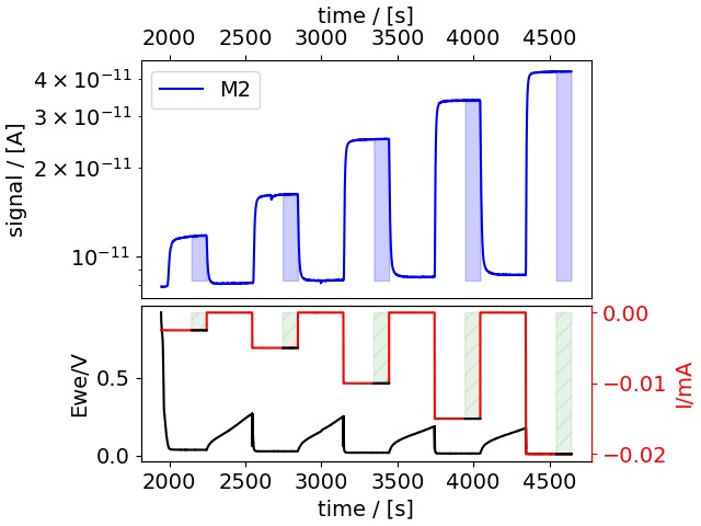
(a) EC‐MS plot during HER
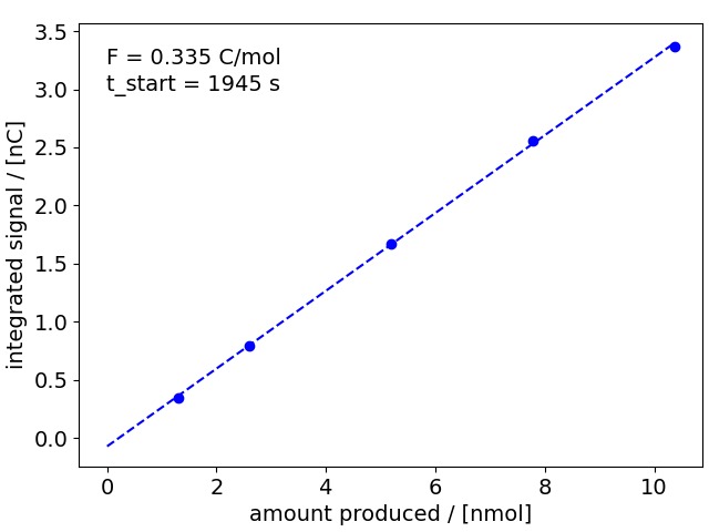
(b) Calibration curve H2
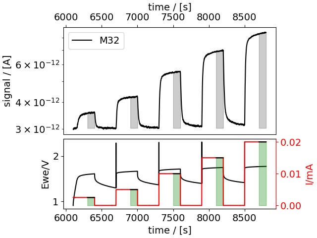
(c) EC‐MS plot during OER
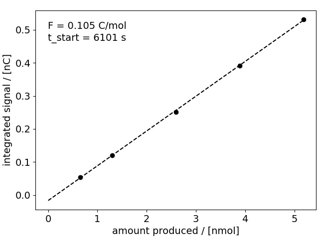
(d) Calibration curve O2
Figure 1: HER and OER sequences and calibration curves with extracted FHER and FOER.
The documentation of this method can be found in the ixdat documentation on the EC-MS module. In the example for HER shown above, we use following syntax to generate the plots shown in Figure 1a and 1b and to calculate the calibration factor for H2:
# first plot the measurement in the time span of the CP sequence:
axes_c = her_meas.plot_measurement(tspan=[1990, 4700],
mass_list=[“M2”])
her_cal = her_meas.ecms_calibration_curve(mol=”H2″,
mass=”M2″, n_el=-2, selector_name=”selector”,
selector_list=[6, 8, 10, 12, 14], tspan_bg=[2900, 3100],
ax=”new”, axes_measurement=axes_c, return_ax=True)
Using the options ”selector_name” and ”selector_list” takes advantage of the potentiostat data containing a cycle/sequence number for the different constant current sequences. This is used to automatically select the time spans of interest, which eases processing of a lot of calibration measurements significantly.
A script to reproduce the above figures will be made available on our website soon.
Partial pressure calibration (semi‐internal calibration)
The limitation of the electrochemical calibration is that it requires that there exists a material that catalyses a reaction to form the analyte of interest at close to 100% faradaic efficiency. To circumvent this problem, a different approach to calibration is possible in the EC-MS: The membrane chip allows to directly introduce calibration gas (mixtures) to the sampling volume via the gas supply system. For highest accuracy, it is recommended to use a calibration gas that is as close as possible to the composition and concentration range expected during the reaction. Depending on the system being studied this can be done by using a bottled pre-mixed gas containing the analytes of interest in the make-up gas, or by mixing the gases from separate bottles before introducing them to the EC-MS. Feel free to contact support@spectroinlets.com for assistance on choosing the right kind of gas calibration set-up for your purpose.
For the measurements shown in the present document, the gases were mixed using two additional MFCs (range 0-20 mL/min and 0-5 mL/min, Alicat Scientific) diluting 100% H2, 1% H2 in He, 20% O2 in He and 100% ethylene (C2H4) with He (5.0). The MFCs were connected with a T-piece after which a filter was placed to ensure thorough mixing of the gases. The outlet of the filter was connected to gas inlet 4 on the setup.
Some of the linearity assumptions discussed in the introductory sections of this document do not hold over the entire concentration range of an analyte. For example, the sensitivity factor for H2 determined at very low H2 concentrations in He is very different from the factor determined using 100% H2. Therefore, we recommend to calibrate using the concentration range expected in EC-MS measurements.
How to do it
If you have a cell, electrode and electrolyte prepared for an electrochemical experiment, and they will not react with or be damaged by the calibration gas, you can use the cell (mounted in the usual way) to close off the chip from the environment while running calibration gases through. Alternatively, it is possible to cover the membrane area of a standard chip with a piece of Kapton tape and use it without a cell on. Note, however, that it is not possible to remove the tape afterwards without damaging the chip. After mounting the chip (or chip + cell), connect the gas (mixture) to one of the gas inlets and prepare the gas lines by repeated pump down and flushing as described in Spectro Inlets’ Technical Note #1 – Gas exchange and EC-MS User Manual. Finally, set the flow to the max. allowed flow for a gas to ensure fast equilibration. (Always keep an eye on the pressure at Pirani 1 and 3 that they do not rise above 0.5 mbar.)
When using a setup with additional MFCs as described above, some extra steps need to be considered. Instead of using MFC2 to regulate the gas flow through the chip, we used the two additional MFCs at the gas cylinders to regulate the flow, while setting MFC2 to “purge” mode. This approach was chosen to ensure that the gas composition was not affected by gas “getting stuck” between the additional MFCs and MFC2. However, this lead to a significant dead volume between the MFCs and the chip, leading to the development of following procedure for setting up a new analyte gas at the external MFC:
- Steady gas flow through the chip was ensured by flowing He from gas inlet 1 through MFC1 at low flow rate (1 mL/min).
- After connecting the analyte gas to the low-flow, external MFC, the dead volume (gas lines to the system, gas manifold, and through MFC2 to V8 set to flow through MFC1) was pumped down through V13 with the external MFC set to max. flow until ca. 25 mbar as shown at the MFC were reached. Before opening V12 and V13, V1 and V14 were closed.
- The external MFC was set to 0 and V13 closed. V1 and V14 were opened to allow for pumping of accumulated gas behind those valves.
- The volume between external MFC and gas bottle was pressurized by briefly opening the valve at the bottle (and making sure to close it again).
- The external MFC was set to max. flow again, and the pump down procedure repeated.
- After pumping down the second time, V13 was closed again, V1 and V14 were opened. MFC2 was set to “normal” mode, flow rate 0.
- The external MFC connected to He (5.0) was set to 20 mL/min and all valves between the external MFC and MFC2 opened.
- After 1.5 min, MFC2 was set to 10 mL/min for 30 s before switching V8. This waiting time was necessary to ensure a high enough pressure at the backside of the chip to prevent breaching. IMPORTANT: Make sure to test the waiting time necessary on your system on a dry chip without droplet or cell on. The pressure at the pressure controller should not drop by more than 50-75 mbar.
- Set the external MFC to 1 mL/min and wait until MFC2 cannot supply the set 10 mL/min anymore.
- Switch the mode of MFC2 to “purge” and set the external MFCs to the ratio necessary to reach the desired analyte concentration
- Wait for the analyte’s MS signal to stabilize.
As the filling of the gas lines this way takes some time, we increased the gas concentration stepwise (starting at the lowest concentration to minimize contamination) without evacuating the system every time. How much time to wait before stabilisation of the MS signal after changing the concentration depends on the analyte and how the gas is connected. In our case, we waited 20 min after changing the settings at the external MFCs. Due to a long gas line between the mix setup and MFC2 including the gas manifold, as the gas bottle was connected through inlet 4, a large volume had to be flushed. Connecting the gases closer to the setup and to gas line 1 or 2 would probably help reducing this time. Nevertheless, if several analyte species should be calibrated for each experiment, it is recommended to buy a pre-mixed gas cylinder containing several analytes to reduce the number of iterations. Also, evaluate if you need a full calibration curve every time or if you can achieve reliable results with just measuring one calibration point per analyte.
Data analysis with ixdat
General
When a gas mixture is flown through the chip and no gas is introduced through the membrane, the gas entering the MS through the capillary is the same composition as the makeup gas. The flux through the capillary can thus be calculated using the capillary equation (Equation (3). Assuming linearity of makeup gas and analyte flux through the chip, which is a reasonable assumption at low analyte concentrations (<10%, better <1%), we can approximate the analyte flux ṅanalyte from the flux of carrier gas ṅcarrier and the known molar fraction of analyte in said gas flow xanalyte), i.e. ṅanalyte = ṅcarrier xanalyte. The calibration factor for the analyte can then be calculated according to Equation (5), essentially in the same way as also done for the electrochemical calibration. Note that for an ideal gas, the molar faction is equal to the volumetric concentration cv,analyte and the ratio between analyte partial pressure and total pressure panalyte/ptotal.
Fcal, partial pressure = ĪMS / ṅanalyte ≈ ĪMS / (ṅcarrier xanalyte) (5)
Using ixdat
The way to calculate calibration factors from a partial pressure calibration in ixdat is similar to how it is done from EC-MS measurements. There are two methods for gas calibration, a single point method and a calibration curve method. Note, though, that in this case they are not a method of the MSMeasurement object, but rather of an MSInlet object which contains the necessary information on capillary dimensions, temperature and pressure. If a different temperature and pressure than standard conditions (298 K and 10000 Pa) should be used, this can be set when defining the MSInlet object.
To calculate the calibration factor F from a single point of known gas concentration in the chip, the following method can be used:
					my_chip.gas_flux_calibration(measurement, mol, mass, tspan=None,
    tspan_bg=None, ax=None, carrier_mol=None,
    mol_conc_ppm=None):
"""
Args:
    measurement (MSMeasurement): The measurement with
        the ms_calibration data
    mol (str): The name of the molecule to calibrate
    mass (str): The mass to calibrate at
    tspan (iter): The timespan to average the signal
        over. Defaults to all
    tspan_bg (iter): Optional timespan at which the
        signal is at its background.
    ax (matplotlib axis): The axis on which to indicate
        what signal is used with a thicker line.
        Defaults to None.
    carrier_mol (str): The name of the molecule of the
        carrier gas if a dilute analyte is used.
        Calibration assumes total flux of the capillary
        is the same as the flux of pure carrier gas.
        Defaults to None.
    mol_conc_ppm (float): Concentration of the dilute
        analyte in the carrier gas in ppm. Default None.

Returns MSCalResult: a ms_calibration result containing
    the sensitivity factor for mol at mass
"""
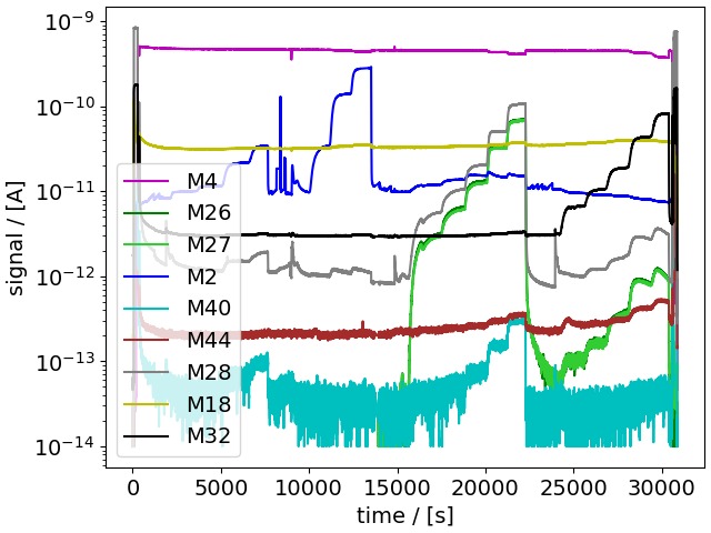
(a) MS signals vs time during gas changes
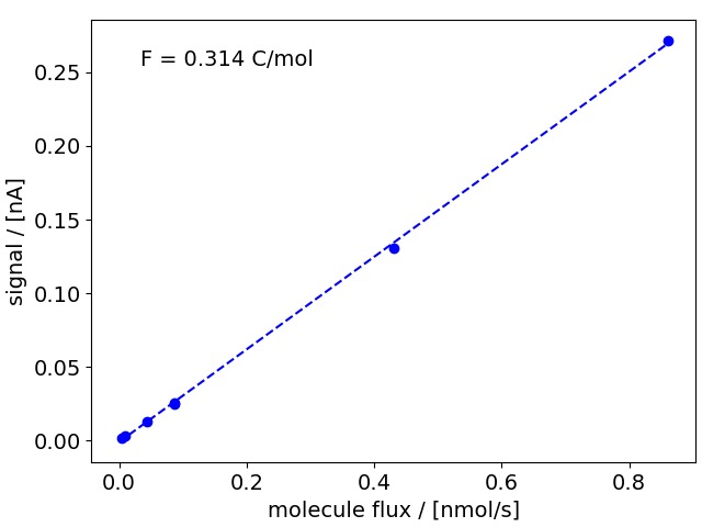
(b) Calibration curve H2, M2
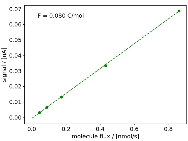
(c) Calibration curve C2H4, M26
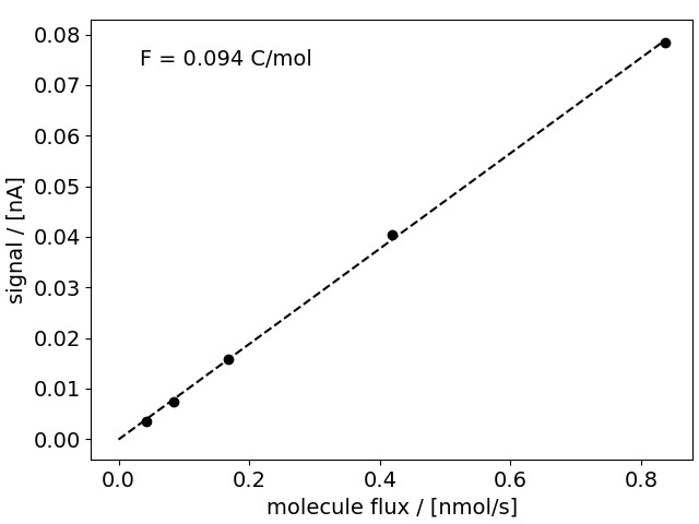
(d) Calibration curve O2, M32
Figure 2: Gas calibration sequence and calibration curves with extracted F. Spikes and irregular variations in the M2 signal between the concentration-step-changes are due to evacuation of the system in between, which can lead to a short-term increase of the pressure in the MS chamber, which reversibly alters the response. The MFC supplying the calibration gas was not purged very well after using C2H4, a gas that adsorbs well to tubing, therefore the ethylene-related signals (M26, M27, M28) also increased during the O2 calibration. This should ideally be avoided by taking more time to repeatedly flush and evacuate the MFC between gases.
					    ax (matplotlib axis): The axis on which to indicate
        what signal is used with a thicker line.
        Defaults to None.
    carrier_mol (str): The name of the molecule of the
        carrier gas if a dilute analyte is used.
        Calibration assumes total flux of the capillary
        is the same as the flux of pure carrier gas.
        Defaults to None.
    mol_conc_ppm (float): Concentration of the dilute
        analyte in the carrier gas in ppm. Default None.

Returns MSCalResult: a ms_calibration result containing
    the sensitivity factor for mol at mass
"""
If more than one concentration point (or alternatively pressure point) is available for an analyte, following method can be used (for detailed documentation look here):
					my_chip.gas_flux_calibration_curve(measurement, mol, mass,
    tspan_list=None, selector_list=None, selector_name=None,
    carrier_mol=None, mol_conc_ppm=None, p_inlet=None,
    t_steady_pulse=0, tspan_bg=None, ax='new',
    axes_measurement=None, return_ax=False)
In the example for H2 calibration shown above, we use following syntax to generate the plots shown in Figure 2b and to calculate the calibration factor for H2:
					all_H2_cal = mychip.gas_flux_calibration_curve(
    full_data,  # MSMeasurement object with calibration data
    mol="H2",
    mass="M2",
    tspan_list=[
        [3037, 3504],
        [4439, 4956],
        [6038, 6456],
        [7243, 7538],
        [10760, 11031],
        [11941, 12236],
        [13023, 13367],
    ],
    carrier_mol="He",
    mol_conc_ppm=[500, 1000, 5000, 10000, 10000, 50000, 100000],
    tspan_bg=[1750, 1950],
    return_ax=True
)
How to use the calibration factor
General
Determining the calibration factor is of course only the first step in the calibration of EC-MS data. To obtain calibrated MS data in mol/s, first the background signal needs to be subtracted. This is especially important for analytes such as O2, N2 or H2 where the background is significant due to the abundance in the atmosphere or as a side product from aqueous electrolyte. After background subtraction, the signal is multiplied with the calibration factor Fcal to calculate the molecule flux to the capillary.
Figure 3 compares two EC-MS plots of cyclic voltammograms recorded on polycrystalline Pt between the OER and HER calibration steps before and after calibration using the calibration factors determined from OER and HER calibration for O2 and H2, respectively.
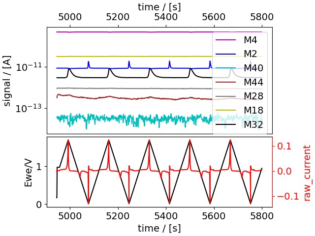
(a) EC‐MS plot vs. time, uncalibrated
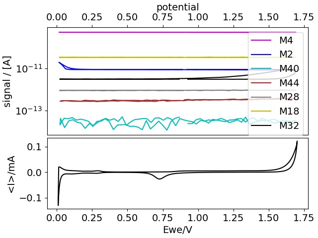
(b) EC‐MS plot vs. potential, uncalibrated
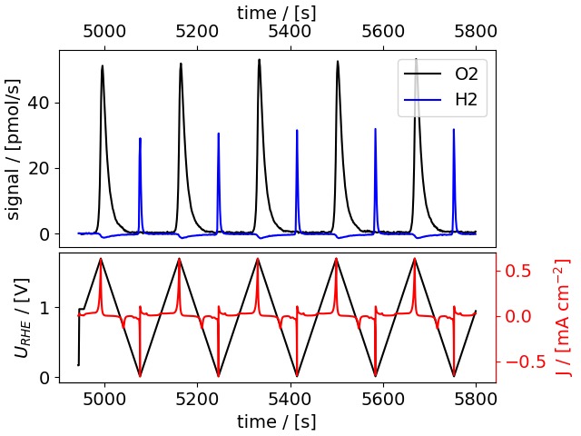
(c) EC‐MS plot vs. time, calibrated
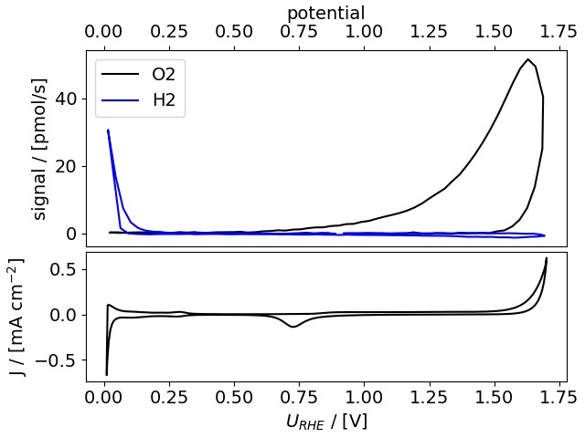
(d) EC‐MS plot vs. potential, calibrated
Using ixdat
Calibration of an (EC)-MS dataset in ixdat is done as follows:
					# use the calibration to calibrate the data of an
# ECMSMeasurement obj.
# OER_cal and HER_cal are MSCalResult objects
cv_sequence.calibrate(ms_cal_results=[OER_cal, HER_cal],
    RE_vs_RHE=0, A_el=0.196)
The plots containing the calibrated data can then be generated with following methods (resulting plots shown in Figures 3c and 3d):
					cv_sequence.plot_measurement(
    mol_list=["O2", "H2"], tspan_bg=[4950, 4970], logplot=False,
    unit="pmol/s"
)
# plot one of the CVs (the 2nd out of 5) vs potential.
cv_sequence[2].plot_vs_potential(
    mol_list=["O2", "H2"], tspan_bg=[5125, 5135], logplot=False,
    unit="pmol/s"
)
Additional remarks
Calibration frequency and expected variability of Fcal
As calibration for an analyte is an additional step in an experiment and requires some time, determining the right calibration frequency in order to achieve reproducible results is important.
In general, MS signal intensity will change over time as the components in the MS age. Also, the signal intensity differs significantly when using different MS hardware, or at different MS settings. Even without changing settings, as mentioned in the theoretical part of this document, when using the electron multiplier (CEM) the signal will decrease significantly already over short periods of time (on the order of 1 h). When using the Faraday cup, the calibration factors stay the same over longer periods of time. Nevertheless, if you’re trying to achieve the most accurate results, even with the Faraday cup, we recommend to run a calibration for the compounds of interest before every important measurement. When choosing to use the CEM, frequent calibration is a requirement and linear interpolation between beginning and end of measurement is recommended.
As with any experimentally determined value, even when repeatedly measuring the calibration factor on the same instrument, using the same technique and the same settings, a certain variability is expected. When preparing this document, we carried out 13 and 15 measurements of FOER and FHER, respectively, varying the calibration method (electrochemical or partial pressure), the chip (i.e. difference between nominal and actual capillary size), and whether the chip was closed with a cell or Kapton tape for partial pressure calibration.
Overall, we see a standard deviation of 4.5% of the mean for O2 and 3.5% of the mean for H2. While the data shown in this Application Note indicates that the calibration factors determined from partial pressure calibration are lower than those determined using electrochemical calibration for the same analyte, when comparing all O2 and H2 measurements done in preparation of this document, this trend is not confirmed. Within the (limited) number of measurements done, we did not find a systematic contribution to the variability from the three possible factors tested.
Overlapping masses
Ideally, one characteristic mass fragment is chosen for each analyte in the system one is studying. However, often, especially when studying reactions that involve several (organic) molecules, one runs into the problem that there are no such mass fragments that are related to one molecule only. Nevertheless, also in this case it is possible to differentiate the origin of a mass signal by calibrating several mass fragments, looking up the expected fragmentation pattern in a database (for example in the NIST database) and then calculating the contribution of molecule A to mass a by subtraction of the contribution of molecule B to mass a by multiplying the signal at mass b by a factor. Details are out of the scope of this Application Note, but can be found in Soren Scott’s PhD thesis [1].
References
[1] S. Scott, “Isotope-labeling studies in electrocatalysis for renewable energy conversion,” Ph.D. dissertation, 2019.
[2] K. Krempl et al., “Dynamic interfacial reaction rates from electrochemistry–mass spectrometry,” Analytical Chemistry, vol. 93, no. 18, pp. 7022–7028, 2021. DOI: 10.1021/acs.analchem.1c00110.
[3] R. Sander, “Compilation of Henry’s law constants (version 4.0) for water as solvent,” Atmospheric Chemistry and Physics, vol. 15, no. 8, pp. 4399–4981, 2015. DOI: 10.5194/acp-15-4399-2015.
[4] T. R. Henriksen, J. L. Olsen, P. Vesborg, I. Chorkendorff, and O. Hansen, “Highly sensitive silicon microreactor for catalyst testing,” Review of Scientific Instruments, vol. 80, no. 12, p. 124101, 2009. DOI: 10.1063/1.3270191.
[5] U. J. Quaade, S. Jensen, and O. Hansen, “Fabrication and modeling of narrow capillaries for vacuum system gas inlets,” Journal of Applied Physics, vol. 97, no. 4, p. 044906, 2005. DOI: 10.1063/1.1829377.
All data treatment and plotting in this application note was carried out using the open source Python package ixdat, available at https://github.com/ixdat/ixdat.
I left out the page footer (“EC-MS quantification | EC-MS Application Note #2 | v. 1.1 | www.spectroinlets.com, Page 15”) because it’s part of the PDF layout and not page content. In the references, I closed up the page numbers “124 101” and “044 906” to 124101 and 044906.