

Benchmark Measurements
EC-MS Technical notes #2
- Last updated

Experimental Procedure
The system can be characterized by standardized benchmark measurements described in this Technical Note. Caution must be exercised by the user when performing such experiment, as variations in electrode active surface area, electrolyte composition, electrolyte purity, surface cleanliness, etc. may influence the results. However, small adjustments of the electrochemical parameters should allow for reproducing Figure 1 adequately.
We recommend using a polished polycrystalline Pt electrode (PtPoly) for performing this benchmarking procedure. If no PtPoly electrode is available, alternatively, a glassy carbon (GC) electrode can be utilized instead, adjusting the measurement parameters accordingly as described below. When using a GC electrode, it is important to follow the additional guidelines described on page 3.
(i) Start a measurement in Zilien, recording the following masses:
- M2 (H2, signal should scale with hydrogen evolution reaction (HER))
- M4 (He)
- M18 (H2O)
- M28 (N2/CO)
- M32 (O2, signal should scale with oxygen evolution reaction (OER))
- M40 (Ar)
- M44 (CO2, signal should scale with CO2 evolution)
(ii) Start He flow in the chip and wait for signals to stabilize, 10 ml/min at the beginning to clean the line (see gas exchange procedure in the EC‐MS Manual), then it can be reduced to 1 mL/min. He gas purity must be at least N5.
(iii) Mount a PtPoly disk (or GC disk) in the EC‐cell. Make sure the disk and U‐cup are flush with the cell and the cell is dry and cleaned of dust/particulates. Refer to EC‐MS Technical Note #11 for a detailed guide on electrode mounting.
(iv) Mount the cell on the instrument, see EC‐MS Technical Note #11.
(v) Fill the EC‐cell with aqueous 0.1 M HClO4 electrolyte (perchloric acid, analytical grade)
(vi) Fill the glass pipes with the same electrolyte (make sure to avoid bubbles beneath the glass frit)
(vii) Connect glass pipes to the EC‐cell
(viii) Insert a reference electrode in the first glass pipe and connect it to the potentiostat (white lead), ensure it is submerged in electrolyte.
(ix) Insert a counter electrode in the second glass pipe, ensure its surface area is higher than that of the working electrode. A coiled Pt wire or mesh works well.
(x) Program an advanced cyclic voltammetry (CVA) experiment in EC‐Lab, using the following parameters:
- Lower (cathodic) potential limit V1 = 0.05 V vs RHE for Pt (or ‐0.85 V vs RHE for GC)
- Higher (anodic) potential limit V2 = 1.70 V vs RHE (or 1.80 V vs RHE for GC)
- Start CV at 0 V vs ref.
- Record at least 5 cycles
- Scan speed = 20 mV/s
- Current range = 100 µA, Bandwidth = 1
Note all potentials given herein are given relative to RHE, if another reference electrode is used convert correspondingly.
(xi) In Zilien’s measurement tab, click the button “Trigger EC measurement now”
(xii) A plot similar to that in Figure 1a should be observed: The M2 signal should increase during the cathodic peak due to HER for both the GC and PtPoly. In the cathodic regimes the M32 signal should increase due to OER for the PtPoly and the M44 signal should increase for the GC due to the oxidation of the carbon stub, as shown in Figure 1 and Figure 2, respectively. Any carbon impurities on the electrode and in the electrolyte will be oxidized to CO2 during the anodic sweeps, causing an increase in the M44 signal. Note that GC starts oxidizing and releasing CO2 already before OER onset, i.e. no M32 peaks are observed in the given potential range. If cleanliness is poor, the PtPoly system may exhibit variations in the height of M32 signal and CV shape.
(xiii) Program a chronopotentiometry (CP) sequence in EC‐lab using following parameters:
(a)
- 0 µA constant current for 5 min
- Limits Ewe > EM = pass
- Record Ewe every 10 mV or 1 s
- Current range = 100 µA, Bandwidth = 1
(b)
- ‐25 µA constant current for 5 min
- Limits Ewe > EM = pass
- Record Ewe every 10 mV or 1 s
- Current range = 100 µA, Bandwidth = 1
(c) Alternate between the two sequences for at least 3 times.
(xiv) In Zilien’s measurement tab, click the button “Trigger EC measurement now”
(xv) After the experiment, analyse the decay of the M2 signal in between ‐25 µA‐sequences to get a measure of the systems status, as described below.
Additional considerations when using a glassy carbon electrode
When using a GC electrode, cleanliness is crucial for achieving reproducible results. The cell, glass pipes, syringe and all parts in direct contact with the electrolyte need to be acid‐cleaned thoroughly before assembling the cell. We recommend cleaning by immersion in piranha solution followed by thorough rinsing in ultrapure water and heating to ∼70 °C to desorb sulphate residuals. Also the GC electrode itself needs to be cleaned, as GC often contains trace metal impurities which will affect the performance of the electrode (lower onset of HER): We recommend polishing followed by sonication and rinsing in ultrapure water, or even immersion in piranha.
Warning: Piranha solution is corrosive, highly oxidizing and highly reactive. Make sure to follow the Health & Safety measures required at your institution before you start working with it.
Sequential sonication and rinsing in ultrapure water (milli‐Q, 18.2 MΩcm) are can also be very efficient to obtain good cell cleanliness.
The exact potential limit for onset of hydrogen evolution will depend on the cleanliness of equipment, electrode and electrolyte, as well as the electrode manufacturer. When using a GC electrode, adjust the lower potential limit in steps in the range from ca. ‐0.6 to ‐0.9 V vs RHE such as to achieve a total current of ca. ‐0.03 mA at the potential limit.
For the GC system metal hydroxides (especially Pt traces) facilitate HER at lower potentials than shown in Figure 2, i.e. (1) if cleanliness of the system is poor, HER can occur closer to RHE than ‐0.8 V vs RHE. (2) After a few cycles up to the CO2 evolution potential most of the contaminants facilitating HER will have been stripped off the GC surface, thus lowering the potential at which generation of the M2 signal can be observed. (3) After prolonged potential holds at cathodic potentials the GC tends to (re‐)adsorb any (metal)cations from the electrolyte typically plating the GC with elements with a much higher activity towards HER than pure GC. This can be seen in the CP measurements, where the overpotential necessary for maintaining constant HER current decreases with time (Figure 4a). For these reasons, the GC system is in some respects a very good gauge for validating the user’s cleaning procedure for removal of metal contaminants, assuming sufficiently pure GC stubs are available.
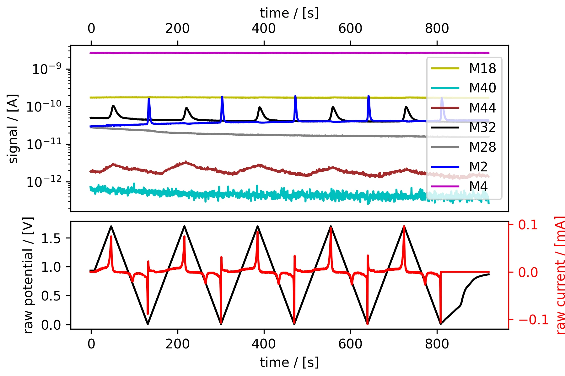
(a) EC‐MS plot of all 5 cycles: Mass spectrometry ﴾top﴿ and electrochemistry ﴾bottom﴿ plotted vs. time.
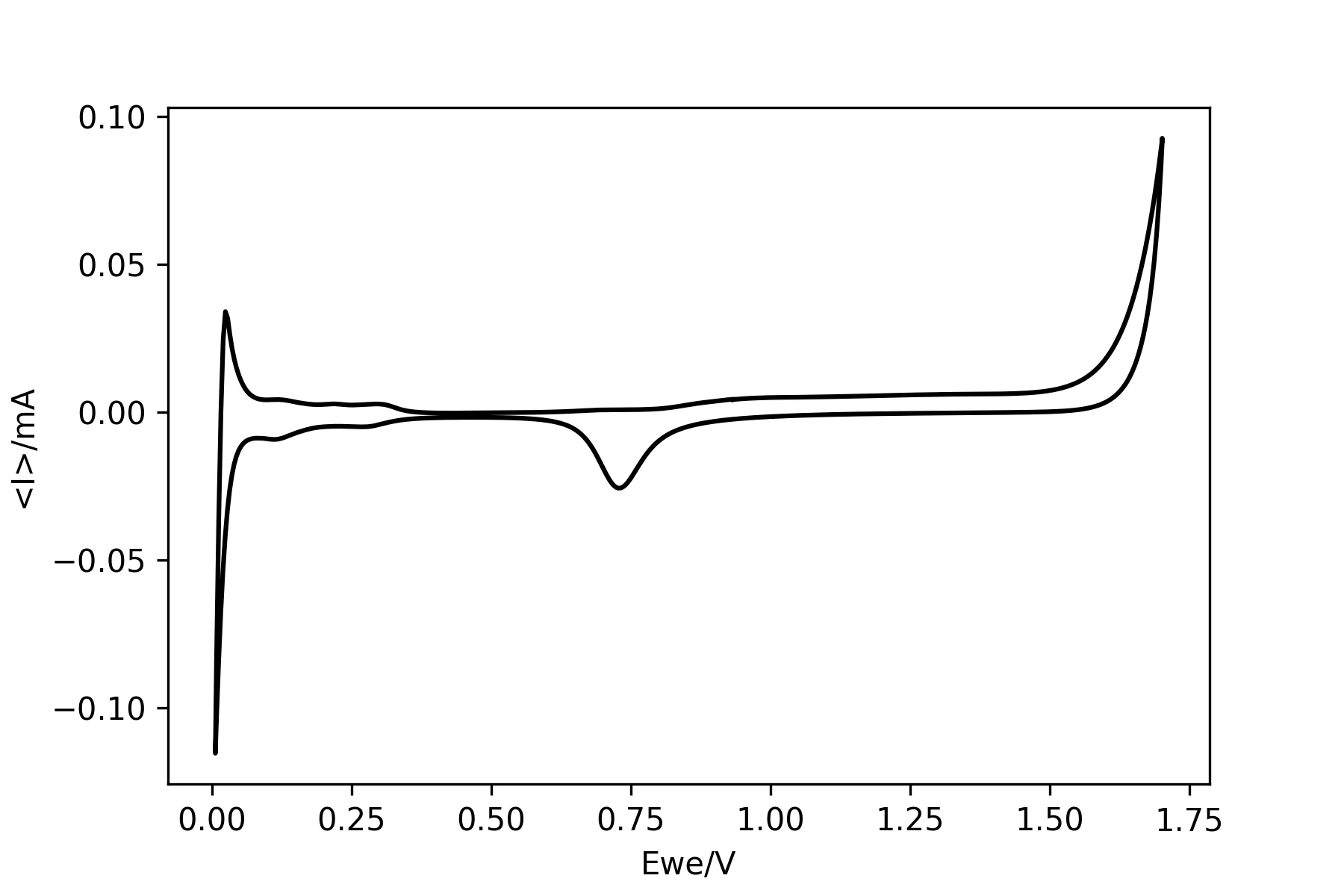
(b) Electrochemical current plotted vs. potential showing a single cycle.
Figure 1: Cyclic voltammogram on a PtPoly electrode. In both subplots, the potential is shown vs. the RHE reference electrode.
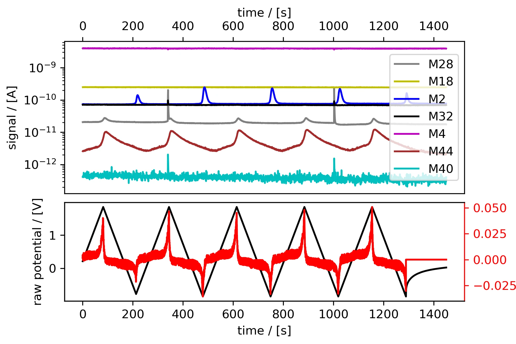
(a) EC‐MS plot of all 5 cycles: Mass spectrometry (top) and electrochemistry ﴾bottom﴿ plotted vs. time.
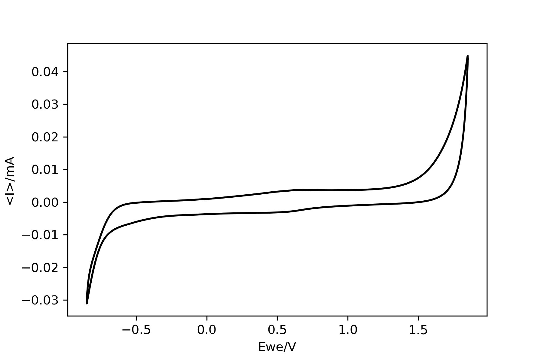
(b) Electrochemical current plotted vs. potential showing a single cycle
Figure 2: Cyclic voltammogram on a freshly cleaned GC electrode. In both subplots, the potential is shown vs. the RHE reference electrode. The signal intensities for the MS signals are higher than for the measurement on PtPoly as shown in Figure 1 as the electron multiplier had been tuned in the between measurements.
Data Analysis
Fitting a single exponential to the decay tails of the M2 signals from the CPs gives an estimate of the decay time constant, according to the following equations:
Y(t) ≡ Y0e−t/τ (1)
Y(t = t0) = 2Y(t = t0 + t1/2) ⇒ t1/2 = ln(2)τ (2)
Where in this case Y is the mass spectrometer signal intensity, t is time, τ is the decay constant, and t1/2 is the decay half‐life constant. Eq. 1 represents a simple exponential decay, whereas Eq. 2 allows to calculate the half‐life associated to such decay, i.e. the time required for the signal to fall to one half of its initial value.
The decay of the analyte signals in the MS is more complex than a simple exponential decay. To obtain a good fit and comparable results it is therefore necessary to limit the fit to the first 5 s of the decay. Typical fitting results and decay constants from the CP experiment are shown in Figure 3 and 4. Following half‐life constants can be extracted for the M2 signal:
t1/2(M2) = 3.8 s (3)
Note that the half‐life constant can vary depending on the alignment of the electrode, the type of electrode and the tuning status of the instrument, as can be seen comparing Figures 3b and 4b.
Note on Data Treatment
All data treatment and plotting in this application note was carried out using the open source Python package ixdat, available at https://github.com/ixdat/ixdat.
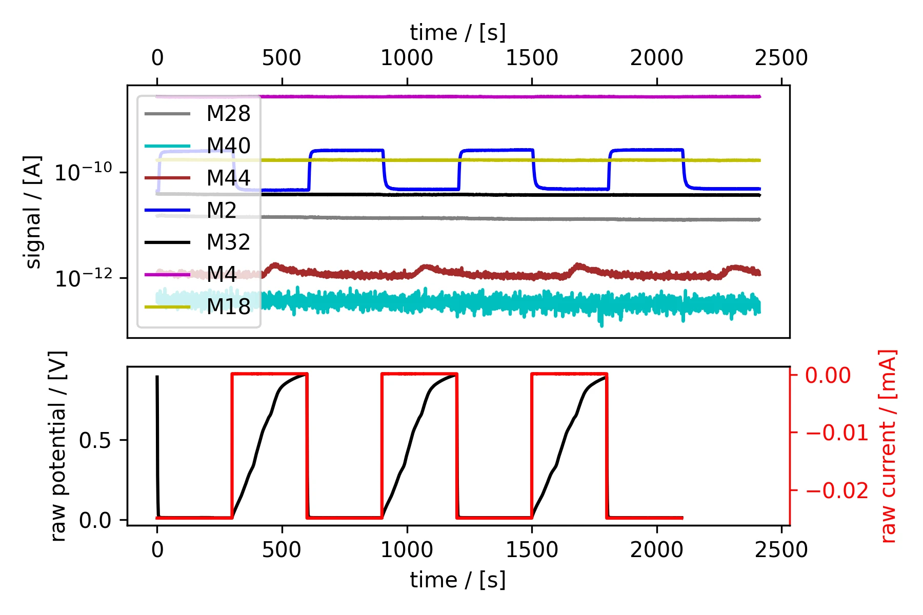
(a) EC‐MS plot: Mass spectrometry (top) and electrochemistry (bottom) plotted vs. time
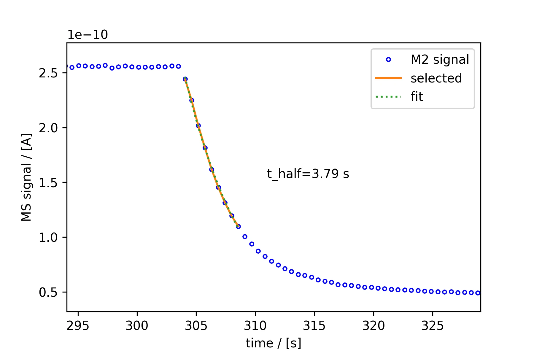
(b) Zoom in to the first decay showing the exponential fit to the first 5 s of the decay.
Figure 3: Sequence of constant current holds (CP experiments) on a PtPoly electrode to determine the decay constant of M2.
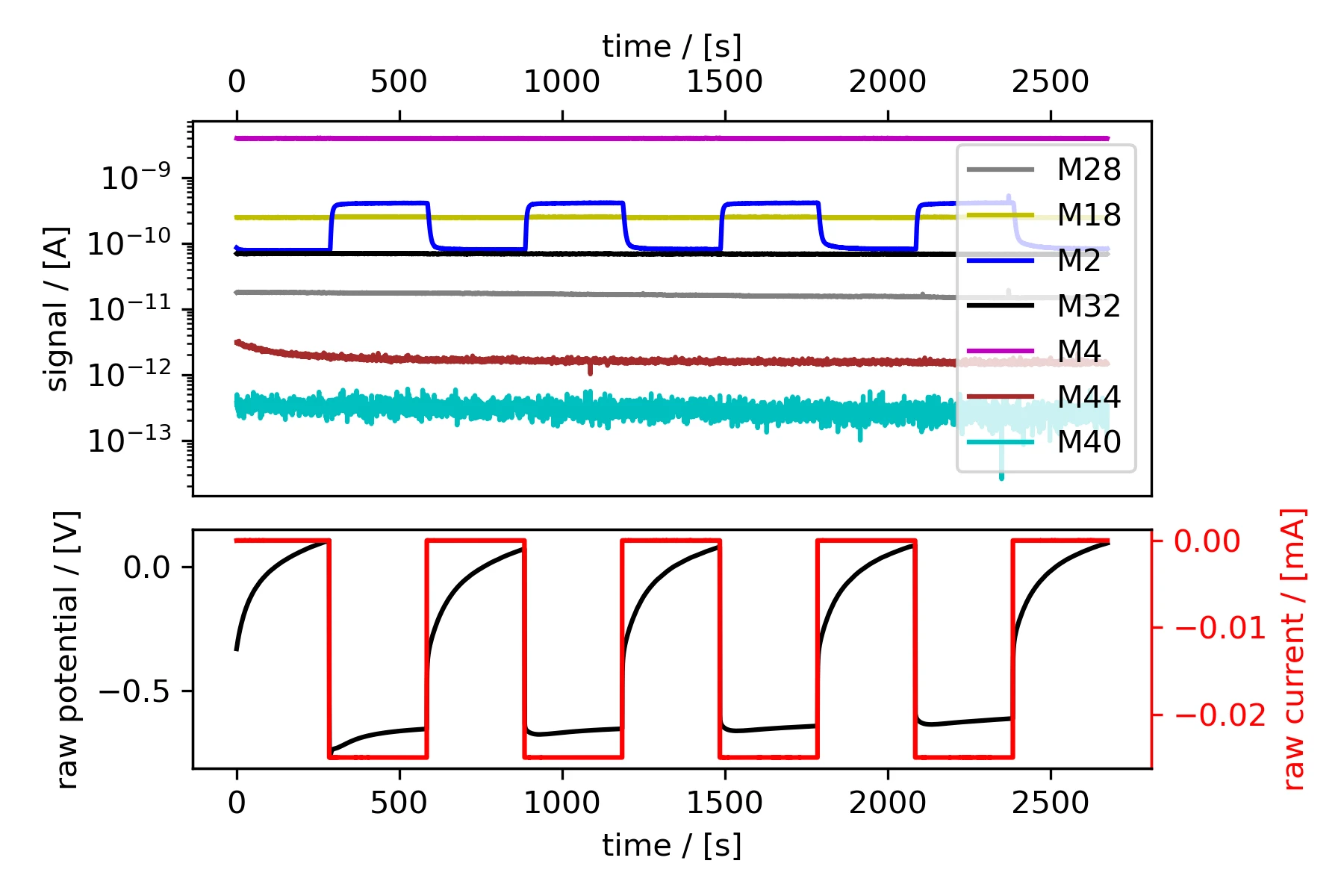
(a) EC‐MS plot: Mass spectrometry (top) and electrochemistry (bottom) plotted vs. time
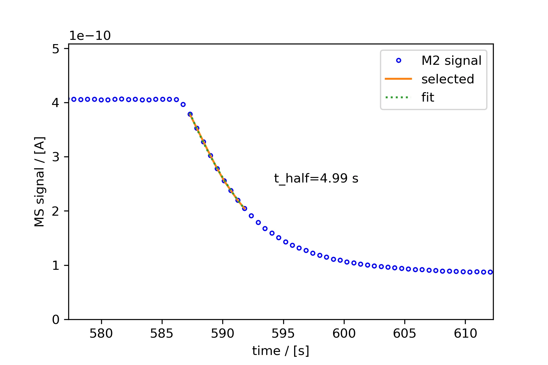
(b) Zoom in to the first decay showing the exponential fit to the first 5 s of the decay
Figure 4: Sequence of constant current holds (CP experiments) on a freshly cleaned GC electrode to determine the decay constant of M2. The signal intensities for the MS signals are higher than for the measurement on PtPoly as shown in Figure 3 as the electron multiplier had been tuned in the between measurements.